There are different types of calculation to measure the
performance of an investment. Choosing the right calculation method is an essential prerequisite for correctly comparing different investments, portfolios or even individual ETFs with each other. There is a choice between the simple rate of return, the money-weighted rate of return and the time-weighted rate of return. In the following, we will highlight the advantages and disadvantages of these three alternatives and explain the differences using some calculation examples.
Time-weighted rate of return
justETF uses time-weighted return to calculate performance on all
portfolio pages and in the
ETF search.
Especially, if you make contributions regularly, this should be the preferred calculation methodology for returns. The reason: The time-weighted rate of return is independent of
cash flows. This provides you with an objective return for each portfolio over any period. Neither the amount nor the timing of payments has an impact on this return calculation. Thus, it is suitable to compare all types of investment products and investment strategies with each other. This allows you to directly compare the time-weighted return of any individual ETF with the time-weighted return of a total portfolio. The time-weighted rate of return is the preferred industry standard and is therefore widely used by investment professionals.
Mathematically, the time-weighted return links geometrically to the daily return factors.
Money-weighted rate of return
In contrast to the time-weighted rate of return, the money-weighted rate of return takes into account the timing and the amount of contributions and withdrawals. When you put money into an investment, in which an investment manager actively controls the cash inflows and outflows, the money-weighted return is the most suitable performance calculation method. Private equity funds or closed-end funds can be mentioned as examples of this. You would also choose the money-weighted rate of return if you do market-timing to measure your success.
If you or your fund's manager are not actively pursuing market-timing, then the money-weighted rate of return over- or underestimates the performance of your investment and thus does not provide a meaningful value to compare your investment success with other investments.
So if you follow a passive
buy and hold approach in your investment, the time-weighted return is the better choice for you to estimate the
performance of your portfolio.
Mathematically, the value-weighted return considers the transactions in the individual periods separately from each other. On the investment amount at the beginning of the first period, an annual return is generated in all periods considered. On the net investment at the beginning of the second period in all periods minus the first, and so on. The annual value-weighted return now indicates a hypothetical constant return that would have resulted in the given terminal value, taking into account all inflows and outflows over time. To determine the value-weighted return of the investment for the entire investment horizon, the annual value-weighted return must then be exponentiated by the number of periods.
Simple rate of return
The easiest way to calculate the return on an investment is to divide the gain or loss of an investment by the amount invested. This calculation is simple and works perfectly for investments without contributions or withdrawals. In all other cases, however, the simple return is not a good indicator for the growth of your portfolio.
Return calculation methods in comparison
To better understand the various calculation methods and their differences, let's look at some case studies below.
Let's assume you invest £5,000 in an ETF portfolio today. For the sake of simplicity, we limit the investment horizon to two years.
If there are no inflows or outflows in the portfolio during the period under consideration, all three calculation methods yield the same result (see case studies 1a), 2a), and 3a)). If, on the other hand, a transaction occurs within the two years we have assumed, the calculated performance of the portfolio will be different - depending on which calculation method is used (case studies 1b), 2b), and 3b)).
Let us consider the following case studies:
- Case 1: Same performance in the 1st and 2nd year (+10% each).
1a) no transaction in the period under consideration
1b) additional deposit of £5,000 after the 1st year
- Case 2: Different performance in the 1st year (+35%) and the 2nd year (+20%)
2a) no transaction in the period under consideration
2b) additional deposit of £5,000 after the 1st year
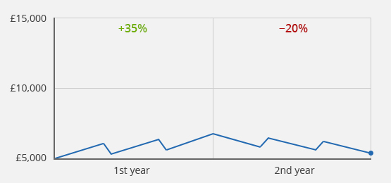
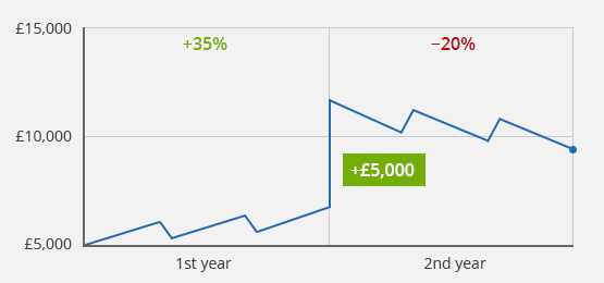
- Case 3: Positive performance in the 1st year (+35%), negative performance in the 2nd year (-20%)
3a) no transaction in the period under consideration
3b) additional deposit after the 1st year
Case 1a): Same performance in the 1st and 2nd year, no transaction
| +21.0% |
Simple return |
| +21.0% |
Money-weighted return |
| +21.0% |
Time-weighted return |
| End value: £6,050 |
Source: justETF Research
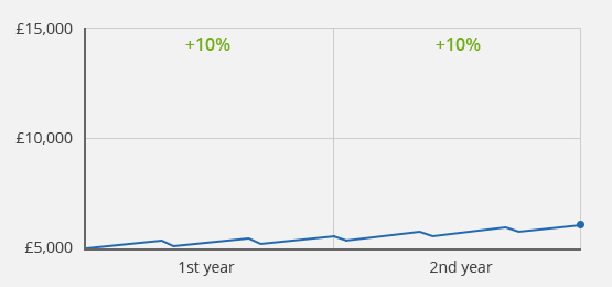
Example 1a): Initial value £5,000/End value after 2 years £6,050/Value development of +10% in the 1st and 2nd year
For the first example, let's assume that the initial investment of £5,000 has become £5,500 after one year. Your investment would therefore have generated a return of 10%. If you're investing for another year and the portfolio increases by +10% in the second year, then your overall return is 21%. Since there were no contributions or withdrawals within the whole period, all three calculation methods provide the same result.
Calculation
Simple return (R_s):
R_s = (6,050 / 5,000) − 1 = 21.0%
Money-weighted return (R_m):
6,050 = 5,000 × (1 + R_w, annual)2
R_m, annual = 10.0% (= money-weighted return, annual)
R_m = (1 + 0.10)2 − 1 = 21.0% (= money-weighted return, total)
Time-weighted return (R_t):
R_t = ((1 + 0.10) × (1 + 0.10)) − 1 = 21.0%
Case 1b) Same performance in the 1st and 2nd year, deposit after the 1st year
| +15.5% |
Simple return |
| +21.0% |
Money-weighted return |
| +21.0% |
Time-weighted return |
| End value: £11,550 |
Source: justETF Research
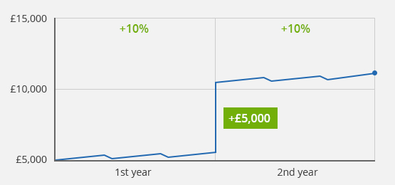
Case study 1b): Initial value £5,000/deposit of £5,000 after the 1st year/final value after 2 years £11,550/value development of +10% in the 1st and 2nd year
What does it mean, if you contribute another £5,000 after one year to this strategy? The performance according to the simple return calculation is now 15.5%. This would mean your investment has underperformed, only because you have contributed additional money after one year. Of course, this is not the case. In this case, the simple return calculation is not suitable.
Because the performance in both years is equal, the money-weighted and time-weighted returns provide the same result. The timing of the contribution does not have any effect.
Calculation
Simple return (R_s):
R_s = (11,550 / 10,000) − 1 = 15.5%
Money-weighted return (R_m):
11,550 = (5,000 × (1 + R_w, annual)2) + (5,000 × (1 + R_w, annual)1)
R_m, annual = 10.0% (= money-weighted return, annual))
R_m = (1 + 0.10)2 − 1 = 21.0% (= money-weighted return, total)
Time-weighted return (R_t):
R_t = ((1 + 0.10) × (1 + 0.10)) − 1 = 21.0%
Case 2a): Different performance in the 1st and 2nd year, no transaction
| +62.0% |
Simple return |
| +62.0% |
Money-weighted return |
| +62.0% |
Time-weighted return |
| End value: £8,100 |
Source: justETF Research
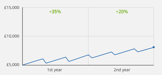
Case study 2a): Initial value £5,000/Final value after 2 years £8,100/Value development of +35% in the 1st year and +20% in the 2nd year
The picture changes, when your portfolio has developed differently in the second year. Suppose, in the first year your portfolio has grown by + 35% and in the second year it has only generated + 20%. If you do not contribute or withdraw any money, then all calculation methods again provide the same result as in example 1a).
Calculation
Simple return (R_s):
R_s = (8,100 / 5,000) − 1 = 62.0%
Money-weighted return (R_m):
8,100 = (5,000 × (1 + R_w, annual)2)
R_m, annual = 27.28% (= money-weighted return, annual)
R_m = (1 + 0.2728 )2 − 1 = 62.0% (= money-weighted return, total)
Time-weighted return (R_t):
R_t = ((1 + 0.35) × (1 + 0.20)) − 1 = 62.0%
Case 2b): Different performance in the 1st and 2nd year, deposit after the 1st year
| +41.0% |
Simple return |
| +56.8% |
Money-weighted return |
| +62.0% |
Time-weighted return |
| End value: £14,100 |
Source: justETF Research
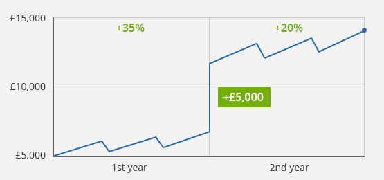
Case study 2b): Initial value £5,000/deposit of £5,000 after the 1st year/final value after 2 years £14,100/value development of +35% in the 1st year and +20% in the 2nd year
However, if a deposit is made into the portfolio in the second period (again, we assume £5,000 for this), the respective results of all three calculation methods differ in this case. In contrast to the previous example 1b), in the case of different performance over time, it very much depends on the point in time at which you make a deposit or a withdrawal. Accordingly, in this case, the value-weighted and the time-weighted return calculation also provide different results. In retrospect, it would of course have been advantageous to directly contribute all money into the portfolio in the first year, since the increase in value was higher than in the second year. For this reason, the money-weighted return results in a lower return of 56.8% over two years. However, if you want to compare the performance of your portfolio with alternative strategies or single ETFs on the
FTSE 100 or
MSCI World, you can only do this by comparing their time-weighted returns.
Calculation
Simple return (R_s):
R_s = (14,100 / 10,000) − 1 = 41.0%
Money-weighted return (R_m):
14,100 = (5,000 × (1 + R_w, annual)2) + (5,000 × (1 + R_w, annual)1)
R_m, annual = 25.2% (= money-weighted return, annual)
R_m = (1 + 0.252)2 − 1 = 56.8% (= money-weighted return, total)
Time-weighted return (R_t):
R_t = ((1 + 0.35) × (1 + 0.20)) − 1 = 62.0%
Case 3a): Positive performance in the 1st year, negative performance in the 2nd year, no transaction
| +8.0% |
Simple return |
| +8.0% |
Money-weighted return |
| +8.0% |
Time-weighted return |
| End value: £5,400 |
Source: justETF Research
Case study 3a): Initial value £5,000/Final value after 2 years £5,400/Value development of +35% in the 1st year and −20% in the 2nd year
Calculation
Simple return (R_s):
R_s = (5,400 / 5,000) − 1 = 8.0%
Money-weighted return (R_m):
5,400 = (5,000 × (1 + R_w, annual)2)
R_m, annual = 3.92% (= money-weighted return, annual)
R_m = (1 + 0.0392)2 − 1 = 8.0% (= money-weighted return, total)
Time-weighted return (R_t):
R_t = ((1 + 0.35) × (1 − 0.20)) − 1 = 8.0%
The calculation methodology may also influence the sign of the calculated return. Thus, it is possible that, for example, the time-weighted return provides a positive result, while the money-weighted or simple return results in negative rates of return. However, this is only possible if deposits or withdrawals have taken place during the period under consideration. Such a case is described in example 3b) below. If no transaction takes place during the period under review, all three calculation methods again lead to the same result (case example 3a)).
Case 3b): Positive performance in the 1st year, negative performance in the 2nd year, deposit after the 1st year
| −6.0% |
Simple return |
| −7.9% |
Money-weighted return |
| +8.0% |
Time-weighted return |
| End value: £9,400 |
Source: justETF Research
Case study 3b): Initial value £5,000/deposit of £5,000 after the 1st year/final value after 2 years £9,400/value development of 35% in the 1st year and −20% in the 2nd year
The fact that the sign of the calculated return can depend on the method used has clear potential for confusion. If you want to compare the performance of your portfolio with an alternative strategy or a benchmark (such as the FTSE 100), the time-weighted return is again the right benchmark.
In case study 3b), the time-weighted return is 8.0%. This is consistent with the value calculated in 3a) - the time-weighted return is therefore independent of the deposit at the beginning of the second year. Assume that the FTSE 100 would have lost −5.0% in the same period. The time-weighted return rightly suggests that in this case, your strategy would have performed much better, +8.0%, than the FTSE 100, −5.0%. Regardless of whether you would have made deposits or withdrawals or not (examples 3a) and 3b)). In contrast, in example 3b), you would not be able to draw this correct conclusion with the simple or the money-weighted return. Instead, the calculated values (−6.0% and −7.9%, respectively) would suggest to you that the strategy you have chosen would have performed worse than the FTSE 100 - a fatal fallacy regarding the quality of your investment strategy, which would only result from the fact that you have made a deposit during the period under consideration.
Calculation
Simple return (R_s):
R_s = (9,400 / 10,000) − 1 = −6.0%
Money-weighted return (R_m):
9,400 = (5,000 × (1 + R_w, annual)2) + (5,000 × (1 + R_w, annual)1)
R_m, annual = −4.1% (= money-weighted return, annual)
R_m = (1 − 0.041)2 − 1 = −7.9% (= money-weighted return, total)
Time-weighted return (R_t):
R_t = ((1 + 0.35) × (1 − 0.20)) − 1 = 8.0%
Conclusion
The above case studies make it clear that only the time-weighted return is independent of inflows and outflows. This enables a direct comparison of different investment strategies or even individual ETFs over arbitrary time periods. For this reason, justETF uses the time-weighted return to calculate the performance of portfolios and ETFs. This allows you to easily and conveniently compare your portfolios with individual indices, objectively and for different time periods.